 |
The Flow Assurance Site |
 |
|---|
1 Introduction
|
This chapter presents some background information, including: |
|
|
|
 When we are likely to encounter multi-phase pipe flow
1.1 Multi-phase flow assurance
1.1.1 General
In the first book in this series, Pipe Flow 1 Single-phase Flow Assurance, we observed that
dealing with single-phase pipe flow is relatively easy in most cases, and the methods for
predicting how the fluid behaves are quite mature. There are still important issues
requiring further investigation, for instance related to something as basic as
determining a pipeline�s friction and thereby its capacity, and progress certainly
continues. But we rarely depend on any groundbreaking new developments in our flow
models to perform the calculations required during planning, design, operator training,
or operation of single-phase pipelines.
The technology for multi-phase flow is in a very different stage of development.
Although multi-phase flow occurs in many industrial processes, methods of
transporting multi-phase fluids through pipelines and wells � which is what this book
is about - has advanced rapidly in recent decades. Multi-phase petroleum wells have
existed for a long time, and multi-phase flow plays an important role in the process
industry, the nuclear industry, and many others. In spite of that, calculation methods
have traditionally been relatively inaccurate and unreliable, at times balancing
somewhere between art and science.

Better flow models are now available, and they are of great help both for predicting
production rates, evaluating gas injection alternatives, avoiding problems with buildup
of hydrates, wax, asphaltenes, scales, or particles. The models are also used to provide
data for corrosion and erosion calculations. The best simulation models are based on
cutting edge technology, incorporating very recent knowledge.
The latest advancements have benefitted and to a large extent also been driven by the
petroleum industry, and it is now possible to transport un-separated gas-oil-water
mixtures over quite long distances. This has already had enormous economical impact
on some offshore developments, and multiphase flow-lines have in some cases replaced
topside offshore installations. That is the case in the Sn�hvit- and Ormen Lange-fields
off the Norwegian coast, where transport distances are well above 100 km. At Tyrihans,
where production was started 2009, the flow-line length is at 43 km relatively moderate
in comparison, but the liquid to gas flow-rate ratio is much higher. The Tyrihans flow-
line connects a new field to existing offshore structures, saving costs by avoiding new
topside structures. At the Con Nam Son-field in Vietnam (outside the range of figure
1.1.1), some processing is done near the wellheads, but only to remove produced water.
Sending gas and hydrocarbon liquid together in a 400 km two-phase flow-line to shore
saves cost both because local processing is reduced (water separation is cheaper than
gas-condensate-water separation) and because one line replaces two by transporting gas
and condensate together.
Further technology improvements are likely to lead to even greater savings for other
fields in the future. In some areas, for instance arctic areas in the north, ice conditions
may mean that multi-phase transportation offers not only the most economical option,
but even the only one technically feasible. Deep-water fields may also pose prohibitive
technical challenges to local separation.
Multi-phase flow is often characterized by liquids and gases occurring simultaneously.
Sometimes there are also solids in the mix. Strictly speaking all of the flow phenomena
surrounding us are multi-phase since no fluid is so clean it does not contain at least
microscopic particles. When we want to describe flow, one of the first challenges we
face is therefore deciding whether we need a multi-phase model. As an example,
consider the earth�s atmosphere. The air contains some water, often in the form of
moisture. As long as both air and water are in gas form, the gas-moisture mixture is
single-phase and behaves quite similarly to dry air. Properties like density,
compressibility, specific heat, and various others are slightly affected by the presence of
the moisture, but the equations describing how it flows or how it exchanges heat with
its surroundings are not. Describing such a fluid is rather similar to describing dispersed
multi-phase flow, for instance small gas bubbles mixed into oil: The gas and oil behave
almost like one fluid, and even though dispersed flow is two-phase, a single-phase
model can for many purposes approximate it quite well.
If air in the atmosphere is cooled down, droplets or ice crystals will sooner or later form,
and the flow becomes two- or even three-phase. Meteorologists can deal with that by
regarding the fluid as single-phase and average all properties accordingly, or they may
use more advanced multi-phase models. Either way, everything becomes more
complicated in that they need to consider such questions as where in time and space the
droplets or ice crystals form, how they are distributed, how large they are, how the
phase shift affects temperature, in addition to various other problems. No model can
realistically describe each droplet or snowflake individually, so some sort of averaging
is needed to simplify. Theory for how to average has a prominent place in some of the
multi-phase literature.
When a scientist has constructed a model to the best of his ability, done calculations and
interpreted the results, he is faced with one final problem: He must evaluate how
reliable the results are. That is also a key requirement when designing a multi-phase
flow-line, and it has many flow assurance implications. It is not adequate to embrace
the results coming out of a commercial simulation tool without asking any critical
questions. The tools currently available are very useful and have user friendly interfaces
(Bratland, 2008), but they can usually not produce simple, reliable answers. The reason
for this is that both the models and the input data rely on simplifications and
approximations. As so often in engineering, it is essential to have a good understanding
of the underlying assumptions and mechanisms and to investigate where the greatest
uncertainties are likely to be found. Cross-checking the results as far as possible, a much
more difficult task in multi-phase than in single-phase flow, is also essential.
In the case of meteorology, the undeniable answer will appear as the weather develops,
and the models can be frequently updated and tuned to improve results. When dealing
with oil and gas developments we are not so fortunate. The first simulations are often
carried out years before the pipeline is even laid, at a time when the available input data
is quite sparse. At the same time the consequences of inadequate predictions can be
very costly and it is certainly possible to end up with a pipeline which cannot do the job
it was designed for. Needless to say, it pays to make the best flow assurance efforts
possible to minimize the risks.
1.1.2 Nuclear reactor multi-phase models
Much of the multi-phase flow theory used in the petroleum industry today rests on
developments done to simulate the coolant water flow around nuclear reactors. Boiling
in the reactor core � as in any steam boiler - leads to two-phase flow. It has long been
known that different sorts of instabilities can occur, and such instabilities can disturb
the heat removal. Various simulation codes have been developed to investigate such
phenomena and other potentially hazardous incidents, for instance loss of feed-water.
Without going into details, it is worth noting that the models developed for nuclear
reactors � models any inquisitive
practitioner in the field of multi-phase
flow is likely to encounter - differ from
those used for petroleum pipelines in
several important ways:
In nuclear reactors, things happen faster than in pipelines (seconds or
minutes, as opposed to hours, days, or weeks). This makes explicit numerical solution
methods and their correspondingly small time-steps more acceptable in the
nuclear than in the petroleum industry. The short reaction times have
implications for other aspects of the theory as well.
Water is a single-component fluid with well-known properties, and in
boilers, it
only occurs in two phases. Well-flow, on the other hand, can contain gas,
oil,
water, as well as sand or other solids, and we therefore sometimes encounter
four-phase flow in the petroleum industry. In addition, it is common that
the
fluid�s composition is poorly known, particularly at early project stages.
The pipes� elevation profiles are very important to how the fluid flows,
and they
are simple and well known in nuclear reactors. That is often not the case in
multi-
phase petroleum flows.
1.1.3 Multi-phase flow in the petroleum industry
In the reservoir in figure 1.1.1, the gas is at the top, and the oil further down. The high pressure can lead to some of the gas being dissolved in the oil, and it may start to be released when the pressure is reduced as the oil travels towards the surface via a borehole. To make reasonable flow calculations, we need to predict boiling and the release of gas dissolved in the oil, and these are phenomena to do with chemical properties, pressure, and temperature.
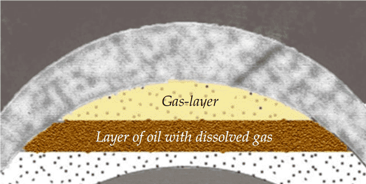
Figure 1.1.2. Petroleum reservoir with gas on top and oil below.
The pressure reduction experienced when hydrocarbons flow towards the wellhead is
partly due to friction and partly due to increased elevation. Gas formation and
expansion directly affect both the pressure and temperature.
One of the most challenging aspects of dealing with multi-phase flow is the fact that it
can take many different forms. In the case of gas-liquid flow, the gas may appear as tiny
amounts of small bubbles in the liquid. That kind of flow occurs when there is relatively
little gas compared to liquid, at the same time as the liquid flows fast enough to create
sufficient turbulence to mix the gas into the liquid faster than the gas can rise to the top
of the pipe.
Figure 1.2.1 illustrates the flow regimes we can encounter in horizontal two-phase gas-
liquid flow. Stratified flow has the strongest tendency to occur in downhill or horizontal
flow with relatively small gas and liquid flow rates. If we increase the gas velocity,
waves start to form, and these waves can get high enough to reach the top of the pipe.
When that happens, the gas is throttled or even blocked for a moment so that the flow
becomes discontinuous, thus leading to the formation of slugs or elongated bubbles.
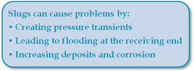
Slugs are generally unwanted because they can create significant pressure fluctuations,
and they can also lead to gas and
liquid arriving at the processing
facilities unevenly, causing tanks
to flood. Since gases have lower
density and therefore lower heat
capacity than liquids, gases cool
faster, so the temperature
reduction during periods of high gas content can more easily cause hydrates to form.
The increased intermittent liquid velocity can also accelerate corrosion.
Figure 1.2.1. Gas-liquid flow regimes in horizontal pipes.
Slugs forming in horizontal pipes of the sort illustrated on figure 1.2.1 iv) are called
hydrodynamic slugs, and tend to be relatively short, typically less than 500 pipe
diameters.
Figure 1.2.2. Terrain slug formation.
Liquid has a tendency to flow towards the low point and block the gas. The gas
pressure builds until the gas reaches the low point and begins to escape into the liquid-
filled uphill section. Once that occurs, the liquid column carried by the gas gets shorter
and shorter, and it becomes easier for the pressure to push it further upwards. As a
result, both the liquid and the gas accelerate out of the pipe.
Figure 1.2.3. Gas-liquid flow regimes in vertical pipes.
The flow regimes occurring in vertical are similar to those in horizontal pipes, but one
difference being that the there is no lower side of the pipe which the densest fluid
�prefers�. One of the implications this has is that stratified flow is not possible in vertical
pipes.
Simulating pipes of any elevation involves determining what kind of flow regime we
are facing as well as doing calculations for that particular regime. Flow regime maps of
the sort shown in figure 1.2.4 are useful when we want to gain insight into the
mechanisms creating the flow regimes.
Figure 1.2.4. Example of steady-state flow regime map for a horizontal pipe.
We see that for very low superficial gas and liquid velocities the flow is stratified. That
is not surprising: As the velocities approach zero, we expect the pipe to act as a long,
horizontal tank with liquid at the bottom and gas on top. If we increase the gas velocity,
waves start forming on the liquid surface. Due to the friction between gas and liquid,
increasing the gas flow will also affect the liquid by dragging it faster towards the outlet
and thereby reducing the liquid level. If we continue to increase the gas flow further,
the gas turbulence intensifies until it rips liquid from the liquid surface so droplets
become entrained in the gas stream, while the previously horizontal surface bends
around the inside of the pipe until it covers the whole circumference with a liquid film.
The droplets are carried by the gas until they occasionally hit the pipe wall and are
deposited back into the liquid film on the wall. We will later learn how to model this
process.
Characterizing flow regimes from visual observations in the laboratory is complicated
as well, and the transitions are difficult to define accurately. To make matters worse, the
flow regimes in figures 1.2.1 and 1.2.3 are not the only ones one may include when
defining horizontal and vertical gas-liquid flow. Different researchers define different
number of flow regimes during laboratory categorization, and the number of regimes
implemented in simulations models is sometimes kept lower for simplicity. The flow
regime selection shown here constitute therefore only one example of how they may be
defined. Predicting the flow regime can be the least accurate part of multi-phase flow
calculations.
Sometimes we must deal with multi-phase flow in annular cross-sections. The
phenomena and flow regimes encountered in such cases are principally the same as in
pipes, but as explained in Pipe Flow 1, the frictions tend to be higher. The flow regime
changes happen under somewhat different superficial velocities in annular compared to
normal pipe flow.
Three phase flow is most often encountered as a mixture of gas, oil and water. The
presence of sand or other particles can result in four-phase flow, or we may have three-
phase flow with solids instead of one of the other phases. Although sand has the
potential to build up and affect the flow or even block it, the most common situation if
sand is present is that the amounts are tiny. If we keep the velocities high enough, the
sand is quickly transported out of the system, and we can often get away with
neglecting the particles in the flow model. Instead, it is only taken into account in
considerations to do with erosion or to establish minimum flow limits to avoid sand
buildup. The three-phase flow our simulation models have to deal with are therefore
primarily of the gas-liquid-liquid sort, and sand is only included � if at all - indirectly.
Creating flow regime illustrations similar to those for gas-liquid flow in figures 1.2.1,
1.2.3, and 1.2.4 is very difficult for three-phase flow. Some authors have done so, but
they end up with very complex illustrations of limited validity, and the pedagogical
value is questionable. It may be more convenient to illustrate three-phase flow as shown
in figure 1.3.1.
We can also experience other liquid-liquid flow regimes, and the number of possible
regimes becomes very large when we move upwards in the three-phase diagram. As a
general rule, it is likely the liquids appear as one dispersed in the other if they occur in
very different quantities. In some cases we can get reasonable results by treating the
two liquids as one averaged liquid and reduce the problem to two-phase gas-liquid
flow. Some of the commercial software treats three-phase gas-liquid-liquid flow in this
way in all situations, but it can lead to quite inaccurate results for some flow regimes.
The various challenges involved in flow assurance for single-phase flow was discussed
in Pipe Flow 1. In multi-phase flow, the most important additional challenges are related
to slugging and the various phenomena which can block or even rupture the pipe. They
are more thoroughly treated in later chapters, but some of the main issues are
mentioned below:
For the most part this book follows the definitions laid down in the first book, Pipe Flow
1. Multiphase flow also calls for additional definitions, some because they improve
clarity, while others have become popular for less obvious reasons. This book tries to
avoid jargon deemed to be of the second sort, but with some exceptions for terminology
essential to understanding other relevant publications.
When we have multiple phases passing through a cross-section of the pipe, each phase
can obviously not cover more than a fraction of the area. If, for instance, a fourth of the
cross-section is occupied by gas, we say the gas area fraction (or the volume fraction, since
volume corresponds to area if the length of that volume is infinitely small) or simply the
gas fraction 0.25. If the remaining area is occupied by liquid, the liquid fraction has
to be 1 - 0.25 = 0.75.
In single-phase flow, we often define instantaneous average velocity (the average
velocity at a particular point in time) as volumetric flow Q [m3/s] divided by pipe cross-
sectional area A [m2]. That way, the average velocity directly reflects the volumetric
flow.
We see that the superficial velocity is proportional to the volumetric flow, and it can be
regarded as the average instantaneous velocity the phase would have had if it occupied
the whole cross-sectional area of the pipe. Since it often occupies only part of it, the
superficial velocity tends to be lower than the actual average velocity.
The mixture (average) velocity in a mixture of N phases is defined as:
We sometimes make use of the mixture (average) density, which is defined as:
Other mixture properties or quantities can be defined in a similar fashion.
In this book, pipe is used with a broad meaning and includes what some authors may
call channel, duct, conduit, tube, wellbore, line, riser, or hose. We sometimes also use
flow-line or gathering network to emphasize that we are referring to the pipe(s)
transporting produced gas/oil/water/sand from one or several wellhead(s) to the
processing facility.
In oil-producing wells we sometimes inject gas via annulus to help the
oil rise to the surface. This can improve production rates and prolong
the well�s economical lifespan, but it can also lead to less table flow.
Some of the challenges involved are discussed later.
Keeping in mind that the well may also produce some water and/or
particles, the well�s elevation profile may have horizontal or even
downhill sections, fluid may flow in at multiple locations, and the fluid
composition may change over time, we realize that predicting the flow
accurately can be very difficult.
Processing facilities are often not located by the wellhead, so the fluid
sometimes continues through gathering networks and flow-lines. The
pressures and temperatures in these networks can lead to deposits of
hydrates, waxes, or other solids, and corrosion or slugging can also
cause problems.
Sometimes we encounter multi-phase flow in pipelines carrying what
was intended to be dry gas, and this can lead to similar problems. In less
severe cases it simply results in altered pipe friction or reduced gas quality delivered to
the customer, but the flow can also become truly multi-phase. In oil pipelines, the
presence of gas bubbles, water, or particles can also make the flow multi-phase.
1.2 Two-phase flow
1.2.1 Flow regimes in horizontal pipes
Another extreme occurs if tiny amounts of liquid droplets are carried by the gas. In that
case part of the liquid becomes deposited on the pipe�s surface and moves as a film in
much the same way water moves on the windscreen of a car driving in the rain.
Remember that since pressures can be high in pipelines, the gas density is typically
much higher that what we are used to experience for air, and even moderate gas
velocities can have great impact. Annular droplet flow can be relatively difficult to
model accurately since the model needs to incorporate such effects as how fast the
droplets are torn from the liquid film, how fast droplets settle on the liquid film, and
how the liquid film affects the surface roughness between gas and liquid. In many
cases, however, the resulting accuracy is acceptable for our purpose, since this kind of
flow does not create the same sorts of problems as slugging does. But it can lead to the
various secondary calculations of deposition or corrosion, which use results from the
flow models as their input, becoming less accurate.

1.2.2 Slugging
Another sort of slugs, referred to as terrain generated slugs, form when the pipe�s
elevation profile creates local elevation minima. Terrain generated slugs can have
periods of several hours, and can originate in both wells and pipelines.

Neither the downhill nor the uphill parts need to be as steep as illustrated here, a
degree of elevation can be sufficient for this to happen. It can occur at any low point in
the pipe, it does not have to be near the outlet. Risers may create these sorts of slugs if
the seabed in front of the riser slopes downwards, and some sorts of risers are shaped
like a J or U in order to allow floater movement.
The effect of slugging can be reduced by actively controlling the choke at the riser�s
outlet. Similar techniques have in some
cases succeeded in countering the
adverse effect of well slugs by actively
controlling the wellhead choke.
1.2.3 Flow regimes in vertical pipes

Most of the published measurements have been carried out on horizontal and vertical
pipes, which is also what we have shown flow regimes for here. Pipelines generally
follow the terrain and most often have other inclinations, so the complexity is often
larger than illustrated here.
1.2.4 Flow regime maps
Along the horizontal axis the superficial gas velocity has been plotted. That
parameter is more thoroughly defined later, but for now, let us just consider it a way to
quantify the volumetric gas flow (or, by multiplying with the density, the gas mass
flow). Along the vertical axis we have plotted the superficial liquid velocity. 
If the liquid flow is very high, the turbulence will be strong, and any gas tends to be
mixed into the liquid as fine bubbles. For somewhat lower liquid flows, the bubbles
float towards the top-side of the pipe and cluster. The appropriate mix of gas and liquid
can then form Taylor-bubbles, which is the name we sometimes use for the large gas
bubbles separating liquid slugs.
If the gas flow is constantly kept high enough, slugs will not form because the gas
transports the liquid out so rapidly the liquid fraction stays low throughout the entire
pipe. It is sometimes possible to take advantage of this and create operational envelopes
that define how a pipeline should be operated, typically defining the minimum gas rate
for slug-free flow.
Similar flow regime maps can be drawn for vertical pipes and pipes with uphill or
downhill inclinations. Notice that even though numerous measured and theoretically
estimated such maps are published in literature, and although they can be made
dimensionless under certain conditions (Taitel & Dukler, 1976), no one has succeeded in
drawing any general maps valid for all diameters, inclinations and fluid properties.
Therefore a diagram valid for one particular situation (one point in one pipeline with
one set of fluid data) is of little help when determining the flow regime for any other
data set. That is why we need more general flow regime criteria rather than measured
flow regime maps. 
Another difficulty comes from the fact that measurements, which are most abundant for
small diameter pipes, are hard to scale up to larger diameters. This problem effects both
flow regime determination and the modeling of each specific regime. 1.2.5 Flow in concentric and eccentric annulus
Two-phase flow can also occur when the pipe carries two liquids � oil and water, for
instance - rather than a gas and a liquid. Liquids tend to have more similar density, and
as chapter 13 will reveal, liquid-liquid flow can result in more flow regimes than those
mentioned so far.

1.3 Three- and four-phase flow
1.3.1 Types of three-phase and quasi four-phase flow
1.3.2 Three-phase flow regimes
The diagram has been plotted in three dimensions, one for each phase. The vertical axis
contains the gas superficial velocity as a fraction of the total superficial velocities. That
superficial velocity fraction has been defined so that it becomes 1 for pure gas flow. For
pure liquid (oil-water) flow, which corresponds to a straight line in the oil-water plane,
the gas fraction is zero. Similarly, if the water content is zero, our operation point will
be located somewhere on a line in the gas-oil plane, and so on for zero oil content.
Operation points inside the triangle will correspond to three-phase flow.
The zero oil and zero water content planes in figure 1.3.1 correspond to gas-liquid flow
regimes similar to those discussed in chapter 1.2. In the oil-water plane, the liquid-
liquid mixture can show a very interesting property we have not mentioned yet: The oil
can occur as isolated droplets dispersed in
the continuous water. If we increase the
oil content, the flow can suddenly switch
to the opposite situation in a process
called phase inversion. The dispersion�s
viscosity tends to be quite similar to the continuous phase�s viscosity, which normally is
much higher for oil than for water.
Whether we have an oil-in-water or water-in-oil
dispersion is therefore very important to the mixture�s viscosity, and we can observe
significant viscosity �jumps� when a phase inversion occurs. If we take a look at the
modified Moody diagram, we see that the consequences of using inaccurate viscosity
(and thereby inaccurate Reynolds number) in the friction calculations depend on where
in the diagram our operational point is located � for relatively high Reynolds numbers
and/or high surface roughness, it may have little or no influence.
1.4 Typical flow assurance tasks
Slugs: The challenge is to avoid, minimize, or design the system so that we can live with
slugs.
Hydrates: Hydrates are ice-like structures which tend to form if the temperature falls
below a certain value when gas molecules are in contact with water. We try to avoid
steady-state hydrate formation (hydrates forming under normal circumstances) by
injecting inhibitors, using thermo-insulation or even heating. We also attempt to
optimize cooldown-times, allowing us sufficient time to take action in case of
shutdown, but without increasing costs more than necessary. Achieving acceptable
hydrate avoidance conditions at a minimum cost usually includes simulating the
known or presumed fluid composition for various alternative anti-hydrate strategies
and ranking the results. The solution must be flexible enough to be able to deal with
uncertainties, and remediation methods in case of blockages are also normally
considered.
Wax: Depending on the fluid�s composition, paraffins in the oil can create challenges
similar as for hydrates, the difference being that we may accept steady-state buildup
and simply choose a high enough pigging frequency to scrape out built-up wax before
the layer becomes thick enough to create problems.
Asphaltenes: This is also quite similar to dealing with hydrates or wax, but chemical
properties making it a problem is encountered somewhat less frequently.
Scales: Scale deposits differ from the others mentioned above in that they are inorganic,
come from produced water, and tend to be harder. Like the others, though, they can be
prevented or removed by inhibitors and pigging. Chemicals can also be used to remove
scales.
Corrosion and erosion: External corrosion is almost always of concern to steel pipelines,
but it is beyond the scope of this book. Depending on what the pipe transports, internal
corrosion is frequently also a concern. The chemistry involved in corrosion is very
complex, and it remains a rapidly developing field. Corrosion is strongly affected by
temperature, pressure, and velocity, and corrosion models can take such data from the
flow models and use them as input. Pure erosion is usually not a problem in petroleum
pipelines, but erosion in combination with corrosion can enhance each other to produce
more damage than they would separately. 
1.5 Some definitions
1.5.1 General
1.5.2 Volume fraction, holdup and water cut
Some authors choose to use a different name for liquid fraction and call it liquid holdup
or simply holdup, while sticking to the fraction-terminology in case the fluid is a gas.
The term water cut is also used occasionally, particularly in describing a well�s
production. It means the ratio of water volumetric flow compared to the total
volumetric liquid flow. Gas � if there is any � is not taken into account in this definition.
Note that water cut does not in itself describe how much water there are in the liquid,
since water and the other liquid(s) may flow at different velocities. Water cut refers to
production rate fraction, not volume fraction. 1.5.3 Superficial velocity
In multi-phase flow, the part of the area occupied by one particular phase varies in
space and time, so the flow is no longer proportional to the velocity at a given point. We define the gas�
superficial velocity as: 
1.5.4 Mixture velocity and density


1.5.5 Various sorts of pipes
The multitude of names used to express pipe is worth keeping in mind when searching
for related literature � the term �vertical pipe slug�, say, may not turn up in certain
articles, even if �vertical duct slug� does.